The same multi-vol quant strategy we all love, but now with 2000+ vol signals to choose from.
quant_rv is a daily SPY strategy that uses realized volatility measures of SPY to predict days of lower volatility ahead, that in turn predict positive returns. In the net, quant_rv wins by very modest improvements to the SPY win ratio and by modest improvements to the average win size relative to the average loss size. In previous posts, we’ve shown that quant_rv can beat SPY total return in several key measures, including both annual and risk-adjusted returns, especially when used as a long/short approach that allocates a small percentage of trading days to an inverse SPY vehicle.
In this post, we introduce a new code approach for quant_rv that provides a more flexible way to test different models and produces a strategy with less uncertainty than our former approach. We’re calling it quant_rv_MV5_big to symbolize that it still uses the Multi-Vol 5 approach (5 different vol measures), with the “big” suffix indicating that we can have a huge number of vol signals by combining these 5 vol measures with a significant range of reasonable lookback periods and volatility threshold values. I was calling it _MV5_2k for a while because I was using ~2000 signals, but that was arbitrary. I use 4k now.
Significantly, by using a more complete sampling of the vol signal parameter space we get a more consistent equity curve, and it’s a bit improved over the original MV5 quant_rv results. We were using 20 randomized signals within a very similar parameter space, now we use 4000 samples and the results converge on an outcome with somewhat better performance.
So let’s take a look. In our old code base, we picked random lookback periods from some narrow windows and random vol thresholds from a modest window, and calculated those to generate 20 vol signals… if 1 or more signals were positive for “low vol” (volatility below threshold) then we went long SPY at the open for the next day, and if 0 signals were below threshold we went short SPY (or long SH).
What the code does now is run a custom function to generate a wide parameter space of volatilities (5 vol measures, 22 lookback periods from 4-25 days) and store those in a XTS matrix. Then we run a second function that generates vol signals by comparing those volatilities to a sequence of 37 thresholds (e.g., 0.13 to 0.22 by 0.0025 increments) for a total 4070 vol signals, for each trading day for SPY. Finally, after creating those once, we don’t recreate them each time (leave them in memory in the R environment) but instead use a third function that calculates the sum of signals for each day across all those signals, or any portion of the signals (ie., send a list of signals to sample, like c(1,22,356,1896)). This makes experimentation fast when running in RStudio, just a couple of seconds to run+plot a new model when the XTS matrices are already calculated in the R environment.
You only need to regenerate the vol and signal matrices if you want to vary the parameter space, or start a new R session environment, or update to the latest market data. By default, the code has a "reloadall” variable near the beginning that is set to FALSE | exists(someobj) so that anything in a if(reloadall) section runs the first time, but only reruns if the environment is cleaned, or “someobj” is removed, or FALSE is set to TRUE.
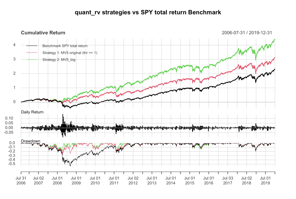
So, back to Figure 1 up there, we see the randomized MV5 “original” equity curve in red, looks just like it did before. It’s a bit more randomized in its current code form, but I may fix that in the future, for fun. In green we have the new MV5 “big” model, using the entire parameter space of 4070 signals. One significant change here between these two is that when using 20 signals, even 1 signal is enough to separate losers from winners (we go long if any 1 or more of the 20 signals is “low”), but with 4000 signals, it’s more profitable to wait to go long until there are about 100 or so signals flashing “low”. It’s a gradual and consistent trend… the more vol signals you sample, the higher the number of “low” signals you should skip before going long. I wrote some suggested numbers in the code for you to play with, if you like.
Other than that, the MV5_big code is practically the same. We don’t pay any attention (at this time) to which vol signals are flashing “low”, or weight some of them more than others. Hell, if you want to do that, you’re more than welcome to, and I’ll bet you can get a lot flashier looking equity curve than I’m showing with a little optimizing in that direction. I don’t think it’s a good idea, particularly, and I’m not interested in joining you in that exercise, but you go right ahead. I think the parameter space I’m using here is pretty broad and by not favoring any particular portion of it, MV5_big is more likely to pick up the right signals going forward when conditions change (and they always change). Optimizing based on the past 15-20 years is likely to bring sorrow unless the next big vol moves develop exactly like the previous ones did, so I’m not optimizing this way.
Here’s another plot, cause I know you’re restless:
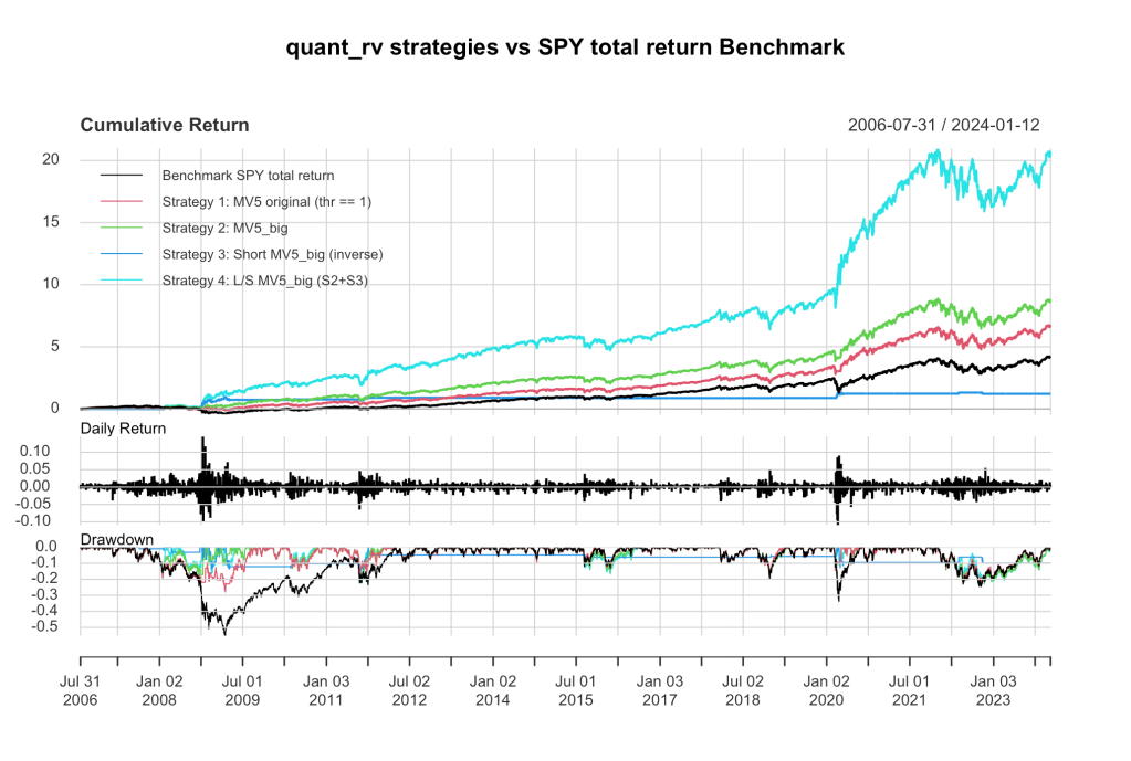
I told you MV5_big uses about 100 “low vol” signals before it goes long. It’s actually coded in there as a random number drawn from 90-110; you can broaden the range, return drops off gently, it seems fairly insensitive. The inverse MV5_big takes whatever that value was (say, 94) and goes short for all the days when there were fewer than that many low vol signals flashing (say, 0-93). This gives a nice robust inverse strategy, and combining the two we stay fully invested long/short with some interesting statistics.
| SPY | S_1 | S_2 | S_3 | S_4 | |
| CAGR | 9.94% | 12.27% | 13.63% | 4.21% | 18.41% |
| StDev | 0.1989 | 0.1587 | 0.1622 | 0.1025 | 0.1917 |
| Sharpe | 0.4999 | 0.7730 | 0.8400 | 0.4109 | 0.9602 |
| MDD | 55.2% | 27.09% | 24.3% | 19.5% | 23.0% |
| Expo | 99.7% | 93.9% | 95.4% | 4.21% | 99.6% |
| Win % | 55.08% | 55.42% | 55.54% | 60.54% | 55.76% |
| Avg Win | 0.770 | 0.703 | 0.715 | 2.257 | 0.786 |
| Avg Loss | -0.843 | -0.752 | -0.761 | -2.353 | -0.821 |
| Win/Loss | 0.914 | 0.935 | 0.939 | 0.959 | 0.957 |
Key in these stats is how modest improvements to sensitive measures make a big difference in strategy outcomes. Except for the the inverse strategy (S_3), the Win % is very little changed, nearly a 1% increase or so wrt the benchmark. But remember – that means ~1% more wins and ~1% fewer losses! The other modest improvement is in the Win/Loss ratio, which improves by a few percent. Those modest improvements team up to yield dramatically better performance by the quant_rv strategies compared to the benchmark.
So… all in all, I think I’m going to put a milestone here in development of quant_rv MV5 at 2.0.0 and say that the latest model is the greatest and from from Jan 16 2024 it’s a wrap and performance from now on for quant_rv_mv5_2.0.0 is out of sample. I’ll specify what I mean is that quant_rv_2.0.0.R in GitHub is the bomb, and further that a “thr2” value of 100 “allvol” (sampling all 4070 signals) should be used for performance testing out of sample. I guess I could call this quant_rv v2, or quant_rv_2.(instead of randomized from 90-100 as in the code) with
I don’t know what I’ll call my next experiments. quant_rv_3 maybe. Sure, that’ll do.
I’ll post performance updates on quant_rv_2 now and then. I think it met my goals, so I’m happy about that.
I’ll stop here for now, the code is posted on GitHub as usual, go play around and let me know what you think, I always appreciate comments here or DM me on Twitter/X if you don’t want your thoughts out in public.

Leave a comment