Elliot Rozner published a blog post recently proposing that one could replace the 40% bond portion of a 60/40 portfolio with a Long/Short equity trend following strategy. Here we’ll put that idea (and his suggested approach) into R using quantmod and examine the components, and finally suggest a free-lunch tweak to improve the risk-adjusted returns further.
Perhaps I’m being a little flip… Elroz carefully steps back and says bonds have their place in your portfolio, of course, of course. But Elroz has an interesting point; as long as the Long/Short trend following strategy meets the expected diversification profile requirements (positive performance, low correlation, and equity crisis protection), who needs bonds in a 60/40? He proposes a simple trend-following strategy using four SMA pairs on SPY (8/32, 16/64, 32/128, 64/256 days), and summing their binary signals (long when short MA > long MA, otherwise short) to scale in and out of the trend strat. So when all four signals are long, trend portion is 100% SPY, when 3 of 4 are long, trend is 50% SPY, 2 long = Hold, 1 long = 50% Short SPY (like in the SH ETF), and all short signals means go 100% Short Spy.
So what’s that look like? I coded it up, and the results look like this:
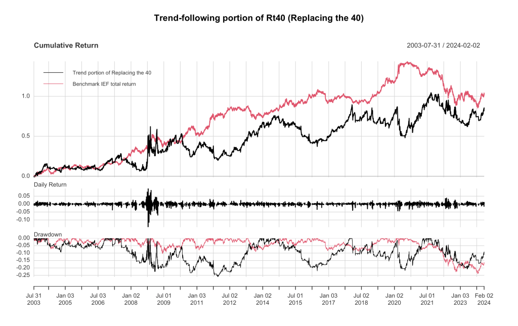
Frankly, the trend following strategy looks kinda sucky. It lags the simple IEF bond benchmark just about the entire time from inception in the early 2000s. In the table below we see the SD is much higher and Sharpe much lower than the bond ETF. True, the max drawdown is roughly the same (except IEF has only drawn down like that once, while trend following went sub-20% several times), and both have significantly negative correlations with SPY. And trend following did pop significantly during the GFC equity crisis in 2008-09, although not in 2020 certainly,
| Trend portion of Replacing the 40 | Benchmark IEF total return | |
| Annualized Return | 0.0308 | 0.0348 |
| Annualized Std Dev | 0.1412 | 0.0686 |
| Annualized Sharpe (Rf=0%) | 0.2178 | 0.5064 |
| Worst Drawdown | 0.2608 | 0.2392 |
| Correlation with SPY | -0.1900 | -0.3046 |
Still, Elroz has a point, it’s an interesting idea. I wonder why he didn’t show these backtests in his blog post? Let’s do the 60/40 thing now and combine them. For simplicity, I’m using daily data, so I’ll just multiply the SPY returns by 0.60 and add the IEF returns by 0.40 and add them, which is like daily rebalancing. And of course I’m not including any fees or slippage or transaction costs at all because fun. And I’ll do the 60/40-Elroz strategy the same way. Here’s the equity curve and matching table:
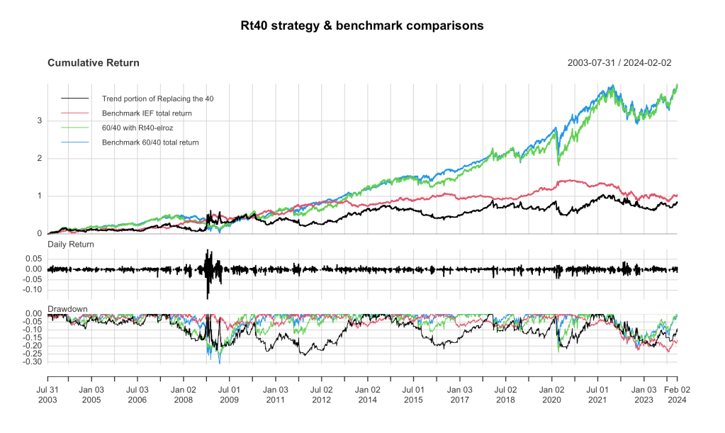
| | 60/40 with Rt40 Elroz | Benchmark 60/40 total return |
| Annualized Return | 0.0817 | 0.0811 |
| Annualized Std Dev | 0.1163 | 0.1079 |
| Annualized Sharpe (Rf=0%) | 0.7019 | 0.7516 |
| Worst Drawdown | 0.2577 | 0.3139 |
| Correlation with SPY | 0.8791 | 0.9702 |
So that’s what we’ve got from Elroz; it’s not quite as good as the 60/40 with this analysis, but part of that (a good part of that) is likely that the Elroz replacement is only fully invested when it’s long 100% (all the trends are up). As Elroz points out in his conclusions, in reality those funds won’t be sitting dormant in cash, they’ll be earning a risk-free rate. And when the trend portion goes short (assuming you’re in a situation where you can actually short SPY instead of having to use a -1x ETF like me), you would have extra cash on hand to earn interest.
Well, as I’ve pointed out here before, that’s not most of us. Most of us have our 60/40 (if we have one) stuck in an IRA where we can’t short SPY, but we’re good for ETFs. And I’m part of the most of us. So I model this as differently. I would use SPY for long and SH for short, and instead of a sweep account where my uninvested cash earns a risk-free rate (I don’t know where to get the data to plug in a time-variant risk-free rate anyway), I’ll use IEF. Because it’s uncorrelated with either SPY or the trend-following strat, it should provide some decent diversification over the long run. So, let’s see what that looks like when we fill the trend-following hold up with IEF:
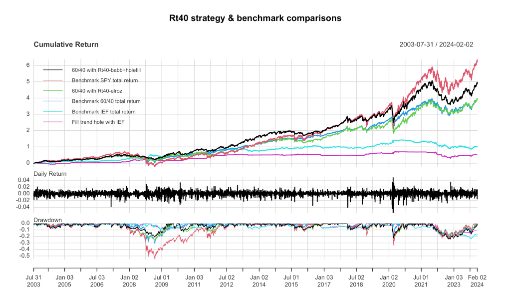
Whoa, not bad, now we’re beating 60/40 soundly on overall return. Let’s look at the stats table:
| | 60/40 with Rt40 Elroz and Holefill with IEF | Elroz again | Benchmark 60/40 total return |
| Annualized Return | 0.9140 | 0.0817 | 0.0811 |
| Annualized Std Dev | 0.1138 | 0.1163 | 0.1079 |
| Annualized Sharpe (Rf=0%) | 0.8027 | 0.7019 | 0.7516 |
| Worst Drawdown | 0.2417 | 0.2577 | 0.3139 |
| Correlation with SPY | 0.8564 | .8791 | 0.9702 |
There ya go, backfilling the uninvested cash with IEF gave us a full percentage point bump, lowered the SD, jumped Sharpe a point, and shaved MDD and the correlation with SPY a tad.
Two more things I’d like to explore. First, is to consider… hmm, just how much IEF hole-filling is optimal? If instead of 40% trend-following where we fill in the hole with IEF, what if we back it off some, and invest even more in IEF, might that improve our Sharpe even more? It would give us some bond exposure over the whole time period, not just when the trend is not-up, so might not be great for overall returns, but risk-adjusted returns might perk up even more.
There’s a couple ways you could do this, but mine is simple, I just add a “shrink” parameter into my strategy where shrink=1.0 means I’m not shrinking the 40% trend-following at all, and shrink=0.0 means I’ve shrunk it to zero and we’re back to a 60/40 SPY/IEF portfolio. Here’s a plot of what the full range of shrinkage from zero to 1 looks like, in risk/reward space:
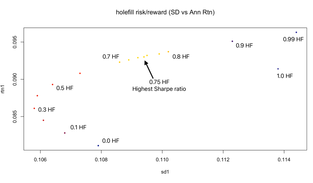
Looks kinda like an efficient frontier plot, maybe, but I don’t think it is, precisely. Like I’ve said, I’m not a quant, but it’s a fun plot to make. Here’s that last table updated to include the 0.75 HF strategy for comparison. Recap first: 0.75 HF is a model with 60% SPY, 30% Trend, 10% IEF, and variable amounts of IEF filling the “hole” created where the Trend model is not fully invested (30% trend is 0.75 “shrink” times the 40% original Trend allocation).
| | 0.75 HoleFill | 60/40 with Rt40 Elroz and HoleFill with IEF | Elroz again | Benchmark 60/40 total return |
| Annualized Return | 0.0930 | 0.9140 | 0.0817 | 0.0811 |
| Annualized Std Dev | 0.1094 | 0.1138 | 0.1163 | 0.1079 |
| Annualized Sharpe (Rf=0%) | 0.8505 | 0.8027 | 0.7019 | 0.7516 |
| Worst Drawdown | 0.2235 | 0.2417 | 0.2577 | 0.3139 |
| Correlation with SPY | 0.8796 | 0.8564 | .8791 | 0.9702 |
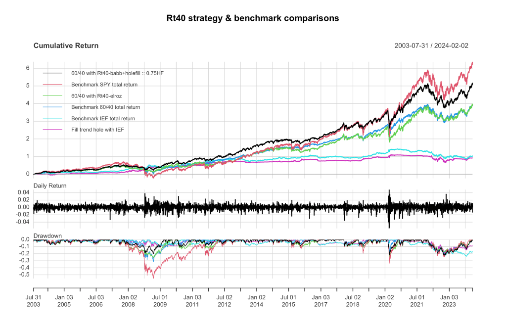
So that’s the best I can do there, and like Elroz hinted at (but didn’t include details), the extra income from filling the hole makes this into a respectable alternative to a traditional 60/40, with higher return and higher Sharpe and even a lower max drawdown over the past 20 years. I throw in one more equity curve, which is almost identical to the last one, but plots the 0.75HF model as the first (black) curve. It even manages to reach a new all-time high in the past week or so, slightly better than the full Elroz with 1.0 holefill we saw above.
One final piece of the puzzle would be to look at the simple components of the Elroz model for investing in trend, and see if his 1, 0.5, 0, -0.5, -1x weights make sense. So I’ve separated them into 5 equity curves for you:
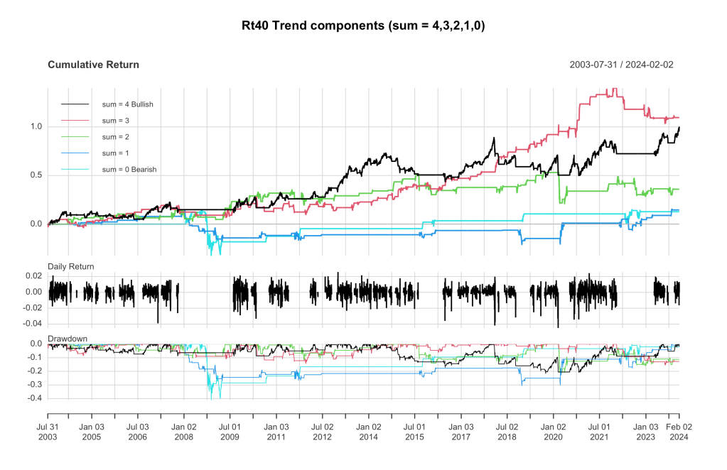
The Daily Return plot in the middle clearly shows the uptrend nature of exposure in the most bullish component of Elroz’ Rt40 trend-following strategy. It’s only invested when all four moving average pairs are bullish, so you can see big gaps for the GFC and the inflation driven bear market we just emerged from, and others as well. Performance of the first two components (sum == 4 and sum == 3) are quite positive with little drawdown, making them fully worthy of Elroz 1x and 0.5x weighting. The two more bearish indicators (sum == 0, 1) are not actual losers over the long term, but certainly have significant drawdowns in the worst equity crises, making them candidates for shorting. There’s maybe some room in here for considering different weights, depending on one’s objectives for using such a moving average scheme.
Personally, I think maybe this model needs MORE moving average pairs, like hundreds or thousands of them. I was enamored with my final version of quant_rv MV5 where it used 4000 measures of realized volatility, and summed the signals very much like this “Replacing the 40” model does, and showed remarkable stability (insensitivity) to changes in the parameterization of the model. Perhaps my own success with quant_rv relates to other recent findings (Bryan et al, 2021) about overparameterization of ML models leading to improved results over more traditional approaches (Box, 1976) of keeping parameterization as simple as possible to avoid overfitting. I don’t know. But I might try to investigate it for a future post.
My code for this post isn’t yet in GitHub, but it will be as soon as I can clean it up a bit. Here’s the code at GitHub (replacing-the-40.R). Nothing fancy in it… Elroz’s SMA strategy is about as easy to code up as any strategy you can find published. I just wanted to get this off my desk. Actually, I haven’t posted code in my blog for a while, so I’ll put the whole thing right here too:
### replacing-the-40.R by babbage9010 and friends
### released under MIT License
# see https://returnsources.com/f/replacing-the-40 by Elliot Rozner
# description:models a 60/40 portfolio using SPY/IEF and then
#  substitutes a simple L/S trend following portfolio for the 40% IEF portion
#  and then riffs on that theme a bit
# originally published Feb 4 2024

# Step 1: Load necessary libraries and data
library(quantmod)
library(PerformanceAnalytics)

#dates and symbols for gathering data
date_start <- as.Date("2002-07-22") #start of IEF
date_end <- as.Date("2034-12-31") #a date in the future
symbol_benchmark1  <- "SPY"  # benchmark for comparison
symbol_benchmark2  <- "IEF"  # benchmark for comparison
symbol_signal1 <- "SPY"  # S&P 500 symbol
symbol_trade1  <- "SPY"  # equity ETF to trade
symbol_trade2  <- "IEF"  # bond ETF to trade

#get data from yahoo
data_benchmark1 <- getSymbols(symbol_benchmark1, src = "yahoo", from = date_start, to = date_end, auto.assign = FALSE)
data_benchmark2 <- getSymbols(symbol_benchmark2, src = "yahoo", from = date_start, to = date_end, auto.assign = FALSE)
data_signal1 <- getSymbols(symbol_signal1, src = "yahoo", from = date_start, to = date_end, auto.assign = FALSE)
data_trade1 <- getSymbols(symbol_trade1, src = "yahoo", from = date_start, to = date_end, auto.assign = FALSE)
data_trade2 <- getSymbols(symbol_trade2, src = "yahoo", from = date_start, to = date_end, auto.assign = FALSE)

#use these prices
prices_benchmark1 <- Ad(data_benchmark1) #Adjusted(Ad) for the #1 benchmark
prices_benchmark2 <- Ad(data_benchmark2) #Adjusted(Ad) for the #2 benchmark
prices_signal1 <- Ad(data_signal1) #Adjusted(Ad) for the signal
prices_trade1 <- Ad(data_trade1) #Ad for our trading
prices_trade2 <- Ad(data_trade2) #Ad for our trading

#calculate 1 day returns (rate of change)
roc_benchmark1 <- ROC(prices_benchmark1, n = 1, type = "discrete")
roc_benchmark2 <- ROC(prices_benchmark2, n = 1, type = "discrete")
roc_signal1 <- ROC(prices_signal1, n = 1, type = "discrete")
roc_trade1 <- ROC(prices_trade1, n = 1, type = "discrete")
roc_trade2 <- ROC(prices_trade2, n = 1, type = "discrete")

# signal_1:  the trend following strategy (per Elroz)
spy8 <- SMA(prices_signal1, 8)
spy16 <- SMA(prices_signal1, 16)
spy32 <- SMA(prices_signal1, 32)
spy64 <- SMA(prices_signal1, 64)
spy128 <- SMA(prices_signal1, 128)
spy256 <- SMA(prices_signal1, 256)
ma_8_32 <- ifelse(spy8 >= spy32, 1, 0)
ma_8_32[is.na(ma_8_32)] <- 0
ma_16_64 <- ifelse(spy16 >= spy64, 1, 0)
ma_16_64[is.na(ma_16_64)] <- 0
ma_32_128 <- ifelse(spy32 >= spy128, 1, 0)
ma_32_128[is.na(ma_32_128)] <- 0
ma_64_256 <- ifelse(spy64 >= spy256, 1, 0)
ma_64_256[is.na(ma_64_256)] <- 0
sums <- ma_8_32 + ma_16_64 + ma_32_128 + ma_64_256
signal_1 <- ifelse(sums == 4, 1, ifelse(sums == 3, 0.5, ifelse(sums == 2, 0, ifelse(sums == 1, -0.5, -1))))
returns_strategy1 <- roc_trade1 * stats::lag(signal_1, 2)
returns_strategy1 <- na.omit(returns_strategy1)
label_strategy1 <- "Trend portion of Replacing the 40"

# signal_2: variable trend following portion, instead of 40%
#shrink - a parameter representing the percentage of trend following to allow in the 40
shrink <- 0.75  # 1 = no shrink (100% trend),  0 = completely shrunken (zero) trend
signal_2 <- ifelse(sums == 4, 1*shrink, ifelse(sums == 3, 0.5*shrink, ifelse(sums == 2, 0*shrink, ifelse(sums == 1, -0.5*shrink, -1*shrink))))
signal_2[is.na(signal_2)] <- 0
returns_strategy2 <- roc_trade1 * stats::lag(signal_2, 2)
returns_strategy2 <- na.omit(returns_strategy2)
label_strategy2 <- paste("Trend portion of Rt40 with shrink:",shrink)

# hole-filling component (IEF into the cash component left by trend following)
# note: this model uses short ETF instead of shorting, so can't use short funds as cash like Elroz suggests
signal_5 <- ifelse( signal_2 > -1 & signal_2 < 1, abs(1-signal_2), 0)
signal_5[is.na(signal_5)] <- 0
returns_strategy5 <- roc_trade2 * stats::lag(signal_5, 2)
returns_strategy5 <- na.omit(returns_strategy5)
label_strategy5 <- "Fill trend hole with IEF"

#signals a-e represent the components of the trend following (sums = 4,3,2,1,0)
signal_a <- ifelse(sums == 4, 1, 0)
returns_strategy_a <- roc_trade1 * stats::lag(signal_a, 2)
signal_b <- ifelse(sums == 3, 1, 0)
returns_strategy_b <- roc_trade1 * stats::lag(signal_b, 2)
signal_c <- ifelse(sums == 2, 1, 0)
returns_strategy_c <- roc_trade1 * stats::lag(signal_c, 2)
signal_d <- ifelse(sums == 1, 1, 0)
returns_strategy_d <- roc_trade1 * stats::lag(signal_d, 2)
signal_e <- ifelse(sums == 0, 1, 0)
returns_strategy_e <- roc_trade1 * stats::lag(signal_e, 2)

#calculate benchmark returns
returns_benchmark1 <- stats::lag(roc_benchmark1, 0)
returns_benchmark1 <- na.omit(returns_benchmark1)
label_benchmark1 <- "Benchmark SPY total return"
returns_benchmark2 <- stats::lag(roc_benchmark2, 0)
returns_benchmark2 <- na.omit(returns_benchmark2)
label_benchmark2 <- "Benchmark IEF total return"
returns_benchmark3 <- 0.6*returns_benchmark1 + 0.4*returns_benchmark2
returns_benchmark3 <- na.omit(returns_benchmark3)
label_benchmark3 <- "Benchmark 60/40 total return"

# Strategy 3: 60/40 with Rt40-elroz
returns_strategy3 <- 0.6*returns_benchmark1 + 0.4*returns_strategy1
returns_strategy3 <- na.omit(returns_strategy3)
label_strategy3 <- "60/40 with Rt40-elroz"

# Strategy 4: 60/40 with Rt40-babb+holefill
returns_strategy4 <- 0.6*returns_benchmark1 + 0.4*returns_strategy2 + 0.4*returns_strategy5
returns_strategy4 <- na.omit(returns_strategy4)
label_strategy4 <- paste("60/40 with Rt40-babb+holefill :: ",shrink,"HF",sep="")


#combine returns into one XTS object, add column names for ploting
comparison <- cbind(returns_strategy1, returns_benchmark2)
colnames(comparison) <- c(label_strategy1, label_benchmark2)
comparison1 <- cbind(returns_strategy1, returns_benchmark2, returns_strategy3, returns_benchmark3)
colnames(comparison1) <- c(label_strategy1, label_benchmark2, label_strategy3, label_benchmark3)
comparison2 <- cbind(returns_strategy_a, returns_strategy_b, returns_strategy_c, returns_strategy_d, returns_strategy_e)
colnames(comparison2) <- c("sum = 4 Bullish", "sum = 3", "sum = 2", "sum = 1", "sum = 0 Bearish")
comparison3 <- cbind(returns_strategy4, returns_benchmark1, returns_strategy3, returns_benchmark3, returns_benchmark2, returns_strategy5)
colnames(comparison3) <- c(label_strategy4, label_benchmark1, label_strategy3, label_benchmark3, label_benchmark2, label_strategy5)

#default chart and stats: uses full data downloaded
#charts.PerformanceSummary(comparison, main = "Golden Death Strategy vs S&P 500 Benchmark - default")
#stats_default <- rbind(table.AnnualizedReturns(comparison), maxDrawdown(comparison))

#trimmed plot and stats
# sdp = start date for plotting
sdp <- "2003-07-31/" #start date for our plot in this blog post
charts.PerformanceSummary(comparison[sdp], main = "Trend-following portion of Rt40 (Replacing the 40)")
stats_gd <- rbind(table.AnnualizedReturns(comparison[sdp]), maxDrawdown(comparison[sdp]))
charts.PerformanceSummary(comparison1[sdp], main = "Rt40 and components")
stats_gd1 <- rbind(table.AnnualizedReturns(comparison1[sdp]), maxDrawdown(comparison1[sdp]))
charts.PerformanceSummary(comparison2[sdp], main = "Rt40 Trend components (sum = 4,3,2,1,0)")
stats_gd2 <- rbind(table.AnnualizedReturns(comparison2[sdp]), maxDrawdown(comparison2[sdp]))
charts.PerformanceSummary(comparison3[sdp], main = "Rt40 strategy & benchmark comparisons")
stats_gd3 <- rbind(table.AnnualizedReturns(comparison3[sdp]), maxDrawdown(comparison3[sdp]))

### add an "exposure" metric (informative, not strictly correct)
exposure <- function(vec){ sum(vec != 0) / length(vec) * 100 }
### and a couple more metrics
winPercent <- function(vec){
  s <- sum(vec > 0)
  s / (s + sum(vec < 0)) * 100
}
avgWin <- function(vec){
  aw <- mean( na.omit(ifelse(vec>0,vec,NA)))
  return( aw * 100 )
}
avgLoss <- function(vec){
  al <- mean( na.omit(ifelse(vec<0,vec,NA)))
  return( al * 100 )
}
extraStats <- function(vec){
  ex <- exposure(vec)
  aw <- avgWin(vec)
  al <- avgLoss(vec)
  wp <- winPercent(vec)
  wl <- -(aw/al)
  return( paste("exp_%:", round(ex,2),  " win_%:", round(wp, 2), " avgWin:", round(aw,3), " avgLoss:", round(al,3), "w/l:", round(wl, 3)) )
}
cat(paste("Model ",shrink,"HF  Rtn: ",stats_gd3[1,1]," SD: ",stats_gd3[2,1]," SR: ",stats_gd3[3,1]," MDD: ",stats_gd3[4,1], sep=""))

#set to TRUE if you want to see these in the console.
if(FALSE){
  print( paste("B1 -", extraStats(returns_benchmark1[sdp]) ))
  print( paste("B2 -", extraStats(returns_benchmark2[sdp]) ))
  print( paste("S1 -", extraStats(returns_strategy1[sdp]) ))
  print( paste("S2 -", extraStats(returns_strategy2[sdp]) ))
  print( paste("S3 -", extraStats(returns_strategy3[sdp]) ))
  print( paste("S4 -", extraStats(returns_strategy4[sdp]) ))
  print( paste("S5 -", extraStats(returns_strategy5[sdp]) ))
  print( paste("_a -", extraStats(returns_strategy_a[sdp]) ))
  print( paste("_b -", extraStats(returns_strategy_b[sdp]) ))
  print( paste("_c -", extraStats(returns_strategy_c[sdp]) ))
  print( paste("_d -", extraStats(returns_strategy_d[sdp]) ))
  print( paste("_e -", extraStats(returns_strategy_e[sdp]) ))
}

# holefill data for plot
# Holefill model means we use Elroz and fill in the unused cash with IEF
# The various models are scaling how much Elroz we use, from 1HF (100% Elroz as 40% of the 60/40)
#   to 0HF, meaning no Elroz, straight 60/40 SPY/IEF
# 0HF means holefilling with IEF
### Note 1: I did this manually while testing, so just dumped in these SD and Rtn values from repeated runs
###   could easily put this in a short loop.
### Note 2: I could have used any scatter plotting, but I like the
###   colors in the default heatscatter so used that for fun
names1 <- c("0HF", "0.1HF", "0.2HF", "0.3HF", "0.4HF", "0.5HF", "0.6HF", "0.7HF", "0.72HF", "0.74HF", "0.75HF", "0.76HF", "0.78HF", "0.8HF", "0.9HF", "0.99HF", "1HF")
rtn1 <- c(0.0811, 0.0828, 0.0845, 0.0861, 0.0878, 0.0893, 0.0908, 0.0923, 0.0926, 0.0929, 0.093, 0.0932, 0.0934, 0.0937, 0.0951, 0.0963, 0.0914)
sd1 <- c(0.1079, 0.1068, 0.1061, 0.1058, 0.1059, 0.1064, 0.1073, 0.1086, 0.1089, 0.1092, 0.1094, 0.1095, 0.1099, 0.1102, 0.1123, 0.1144, 0.1138)
heatscatter(sd1, rtn1, cor=FALSE, main="holefill risk/reward (SD vs Ann Rtn)")
Leave a comment