TL;DR ~ This post explores adding a normalized Average True Range (nATR) measure that behaves in a similar fashion to other volatility measures, including a “low volatile anomaly” and nATR gives quant_rv a nice boost in backtesting performance. Not all goals for quant_rv are met yet, but we’re definitely seeing improvements.
So, I’m getting nearer to a solution for all the quant_rv goals. Progress, not a full and clear solution yet, but it’s got some new promise, it’s offering significantly more hope. Three new codes for this post can all be found at The GitHub (for the statistical plots, heatmap plots and the backtesting) instead of embedding them all here in the blog post.
First up, the goals, again:
- trades popular, liquid ETFs (to allow it to scale meaningfully) with no extra leverage (no 2x or 3x ETFs)
- develops signals based on sensible, logical, statistically meaningful market observations (like realized volatility)
- trades at the next-day Open with signals based on the previous day’s market data (allowing plenty of time for followers to generate signals and place trades)
- unequivocally beats a benchmark of buy-and-hold SPY (including dividends compounded, ie., calculated using Adjusted Close) on all these metrics: Annual Return, Annualized Standard Deviation, Sharpe Ratio, Max Drawdown
- uses the same instruments as the benchmark in order to meet these goals (ie, SPY or derivatives/equivalents, not QQQ or some specific market sector ETF)
- accomplishes its goals without consideration of dividends collected by the strategy (quant_rv gets one hand tied behind its back)
- stretch goal: also performs reasonably well across several different market/ETF areas, to show that it really meets the #2 (sensible) goal above
I’ve chosen to work with realized volatility as my main signal of interest. Low vol market periods tend to move reliably higher, and have a history of that behavior. On a simple level (as shown in earlier posts), simply being out of the market during more volatile periods yields decent risk-adjusted results, getting us part way to our goals. But it definitely doesn’t meet #4 above, unequivocally beating SPY’s performance, at least not the way quant_rv has been approaching it as a strategy. Risk-adjusted, sure, all of the goals really, EXCEPT for Annual Return. So we need something else, perhaps some alternative volatility measure that can give us the performance boost we need.
Our most recent multivol approach for quant_rv uses three different lookback periods for the volatility, with four different vol measures. In this post we’ll explore a fifth vol measure and add it to the mix, and add a fourth randomized lookback period.
Without further ado, we bring ATR into the mix, the Average True Range measure. Clearly meant to be a measure of volatility broadly, ATR is not comparable to our other measures out-of-the-box primarily because it’s a “True Range” measure… it’s not normalized to the price of the equity being measured. A stock priced at $1000 moving $1 in a day may have the same “true range” as a $10 stock moving $1. I say “may have” because the True Range measure is a little trickier than that. Popularized by J. Welles Wilder, he defined it as the range between the High and Low of the day (or bar), but with the twist of instead using the previous bar Close price instead of the Low if the Close was lower than the Low, and/or using the previous Close instead of the High, if the Close was higher than the High. More cleanly, the True Range is the greater of these three:
- High for the day minus the Low for the day
- High for the day minus the Close for the previous day
- Previous Close minus the Low for the day
Another way to look at it is TR uses High minus Low for the day, unless the market gapped up or down. If it’s a gap-up day (and the low never dipped below the previous Close), TR is High minus the previous Close. If the market gapped down (and the High never peaked above the previous Close), TR is previous Close minus Low.
And so the ATR is the average of the True Range over the last X days. J. Welles Wilder used his own custom EMA for the moving average, but a regular SMA, EMA, or ZLEMA (zero-lag exponential moving average) will do the job. I’ve always liked ZLEMA and will use it here. But we also have to normalize it to the signal price (in this case SPY) to get the nATR for our volatility use. With normalization we’re looking at an ATR for that $1000 example stock of about 0.001 and for the $10 stock of about 0.10, sensible numbers (similar to daily percentage move) but not directly comparable to our other volatility measures, where volatility of 0.10 (10%) is quite low. So we’ll be using different thresholds for nATR when we calculate backtests in a little while.
But first, let’s run some of our earlier plots to see how nATR compares to the other vol measures with respect to the distribution of forecasted next-day returns and the “low vol anomaly”. First up is a look at the quantiles associated with a 20-day lookback period nATR. I won’t repost the R code here (but I will put it in the GitHub), but here’s the only new line that matters:
nATR <- ATR(spy_data, n=lookbk, maType="ZLEMA")[ , "atr"] / pricesCl
That says make a XTS object called “nATR” to hold our normalized ATR, and calculate it from the SPY (spy_data) with a 20-day lookback period, normalized to the daily Close (pricesCl). I’m using the unadjusted Close rather than the Adjusted Close because the ATR function uses unadjusted Open and Close values to calculate ATR, so it is best normalized by the unadjusted Close. Add that line and a few supporting lines, and we can generate this plot of risk-adjusted returns:
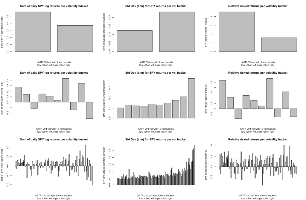
It’s really quite similar to the four previous vol measures (Close-to-Close, Parkinson, Rogers-Satchell, Garman-Klass Yang-Zhang) especially in the remarkably exponential-appearing increase in standard deviation across the vol buckets. The low vol anomaly persists for this new vol measure in both absolute and risk-adjusted returns, much like in the last post.
You’ll recall that we also want to make sure this isn’t just a 20-day fluke. So here’s a color plot of the relative risked return for low vs high vol halves of the data set:
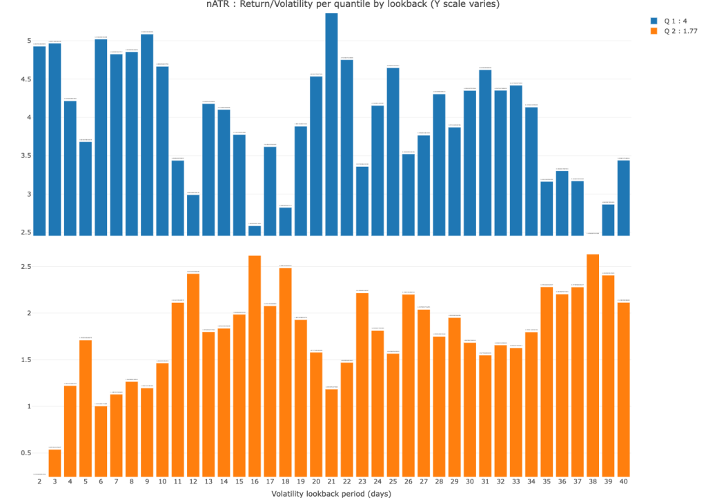
This plot is just like those in the other post, except we’ve run the lookback period up to 40 days (instead of 30) and the vertical scales are variable here (they were fixed at 0-8 range previously). The overall pattern is clear: the low vol (blue) risked returns average significantly higher than the high vol (orange bars) returns, in all but two lookback periods (16 and 38 days), where they are close to parity. So overall, I claim that nATR is a measure of price volatility with comparable behavior (including the low vol anomaly) to the other measures I’ve been using for the purposes I intend, and I’ll add nATR to the mix for some quant_rv backtesting.
As a final comparison between nATR and the other vol measures we’re using, I’ll present four heatmaps similar to the ones used in previous posts. These are similar, but not identical, again because the thresholds required for nATR are different in nature and on a different (smaller) scale from the other vol measures. The TL;DR here is that nATR behaves similarly overall to the others (grossly increasing in exposure and annual return from low thresholds to higher thresholds), but also has some significant variations that make it particularly interesting to us.
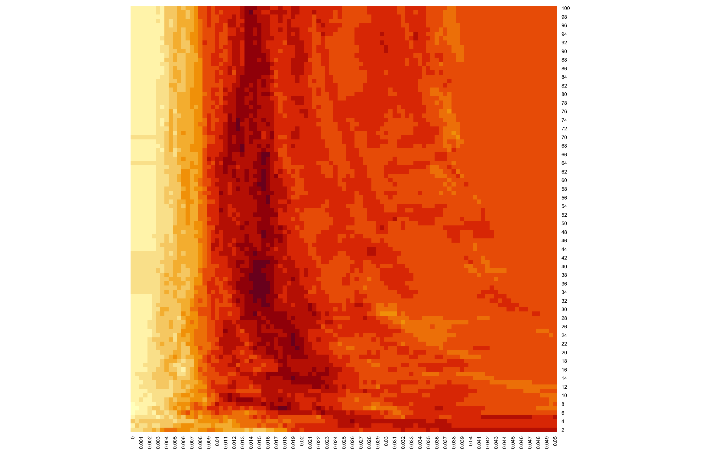
If you’re new to this blog series, these heatmaps reflect backtest results from July 2006 to Dec 2019 for each of thousands of runs covering the parameter space of (1) 2-100 day lookback periods (Y-axis) and (2) 0-0.05 threshold for the nATR vol measure (X-axis, where 0.05 represents nATR value of 5% average true range — quite high), with the simple strategy rule of going Long with SPY at the Open for days where the nATR from the previous Close was below that threshold, and get out of SPY on days where the previous day’s nATR was above threshold. The four heatmaps represent Market Exposure (percentage of market days was the strategy invested Long), Annual Return, Sharpe Ratio, and Maximum Drawdown. The color range displays ten deciles with smaller values represented by lighter colors, and higher values with darker red tones.

Market exposure for nATR displays a pattern of increasing exposure with increasing thresholds, and a slight swing of trends toward the right (higher thresholds) at the shorter lookback periods; this pattern is nearly identical to that of the other vol measures.
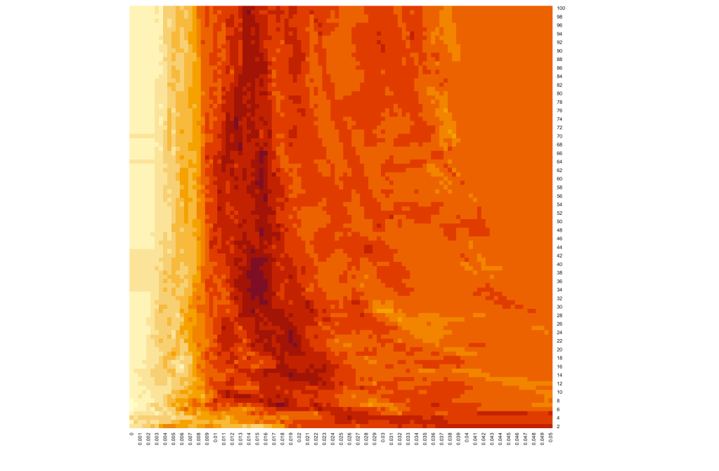
The annual returns pattern displays a pattern of increasing returns with increasing thresholds to a point, then lesser returns at the highest thresholds, and also a broad sweeping pattern of trends from upper left to lower right. This too is similar to the annual returns heatmaps for the other vol measures… except that this nATR pattern seems a bit exaggerated. The highest (darkest) returns area is more concentrated (darker) than the others, and the returns are relatively more modest (lighter shade) in the area of maximum thresholds. This is nice for us, of course… it looks like adding nATR into the multi-vol approach to quant_rv might help bring higher returns while keeping the threshold and market exposure modest.
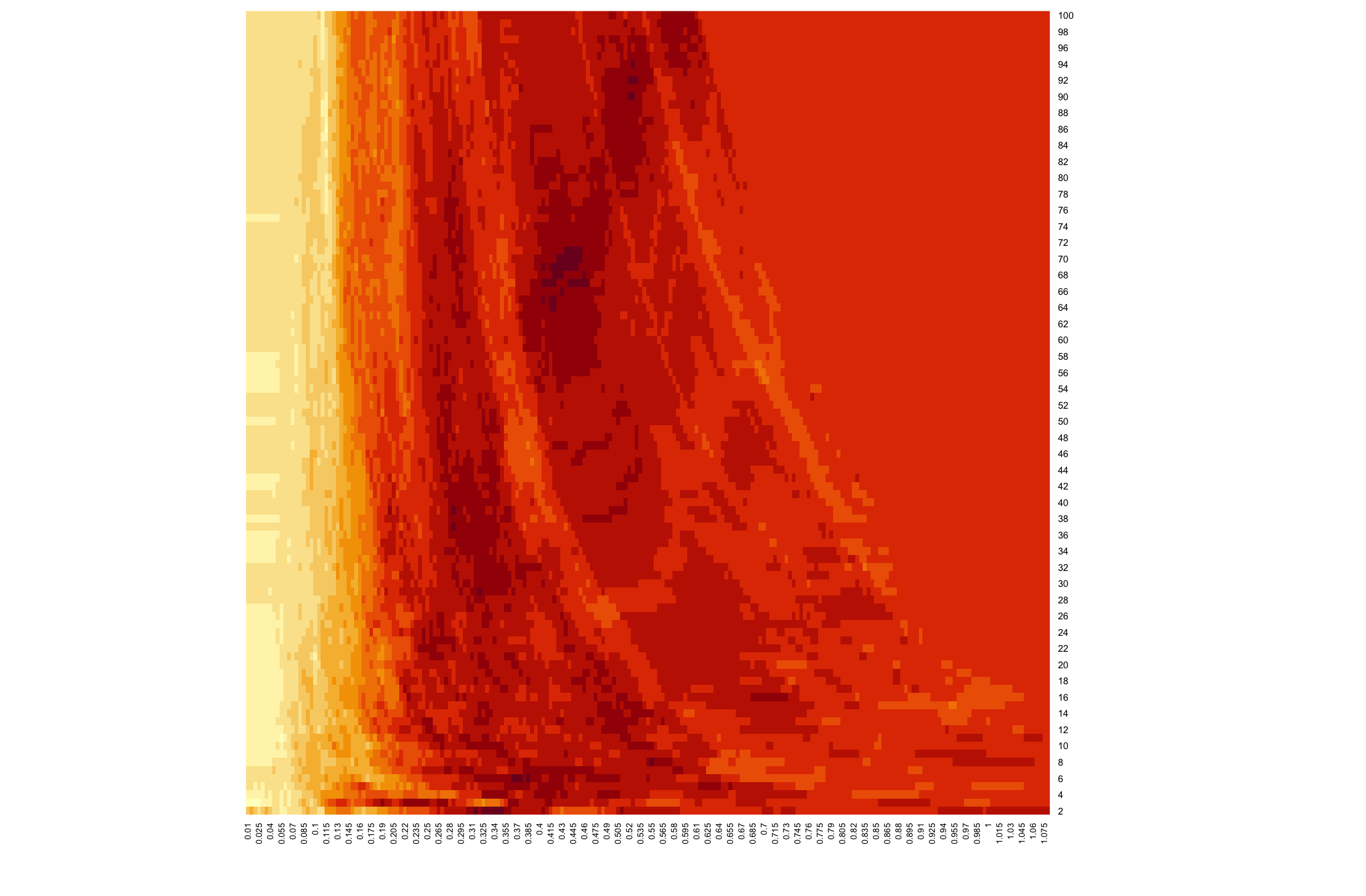
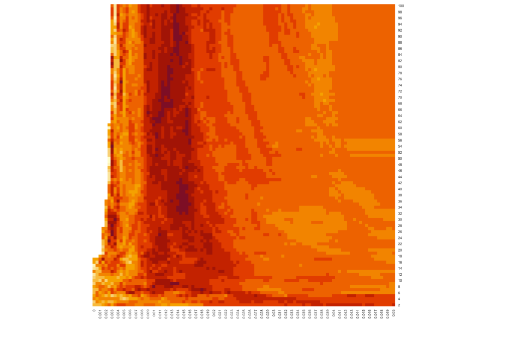
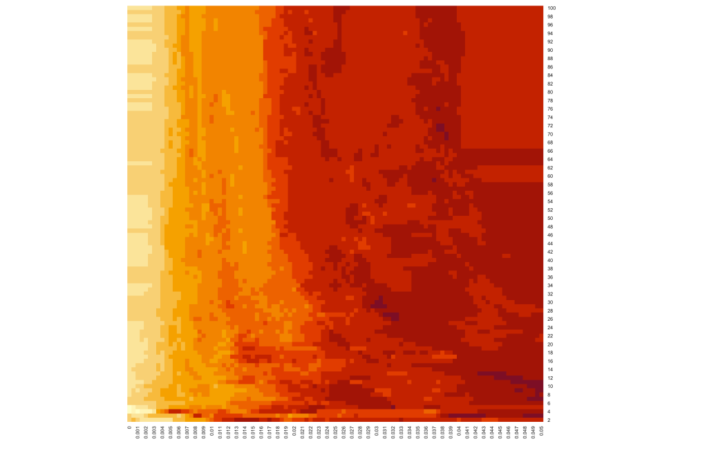
Here’s a look at comparing the nATR heatmap for annual returns with the Close-to-Close volatility heatmap from an earlier post, so that you can visually compare the pattern and trends. The X-axis for these two plots is not directly comparable because the nATR isn’t a “true” vol measure, as discussed above, but the visual comparison is remarkable all the same.
For completeness, here are the other two heatmaps for nATR: Sharpe ratio and Maximum Drawdown. The Sharpe ratio map shows a “hot” area of high Sharpe in sync with the “hot” annual return area. The max drawdown map is similar in style (sweeping arcs of lower/higher maxdd) to the other vol measures.
All in all, nATR seems to stack up reasonably well as a vol measure with similar properties to the other vol measures, and now we’ll add it to quant_rv and see what happens.
Backtesting quant_rv with nATR
The R code for the backtesting is now live on the GitHub, but I’ll just state here that I’ve modified a few bits of the code from the previous “multi-vol” version (described in this post) to utilize in four parts the full range of lookback periods from 4 to 25 days and to include nATR as a measure, and finally to include a second benchmark for comparison, the Open-Open return measured as if it were a buy-and-hold investment but without dividends collected. Thus the new benchmark is a direct comparison to the Open-Open trading approach used by quant_rv in this post, a utilitarian benchmark if you will, whereas the buy-and-hold SPY benchmark is aspirational.
So, for those new to quant_rv or who would like a refresher, the strategy simply goes long at the Open on days when our vol signal is below a given threshold value, and flat when our vol signal is above threshold. The twist is that we calculate the vol signal using four different volatility measures (std deviation of daily Close-Close, plus Rogers-Satchell, Garman-Klass+Yang-Zhang, and Parkinson) with four different lookback periods (picked randomly in zones from 4 to 25 days) for a total of 16 measures. If ANY of the measures says go long, we go long; this approach maximizes market exposure (days invested) and as a strategy says “avoid the market during days where volatility will likely be highest”. In this new version of quant_rv (version 1.3.2 at the GitHub), we’re adding the nATR measures across the same range of lookback periods, and keeping it separate in the code because it uses it’s own much lower threshold range, but then at the end including it the same way as the other measures, giving us a total of 20 vol measures and if ANY one of them says to go long, we go long.
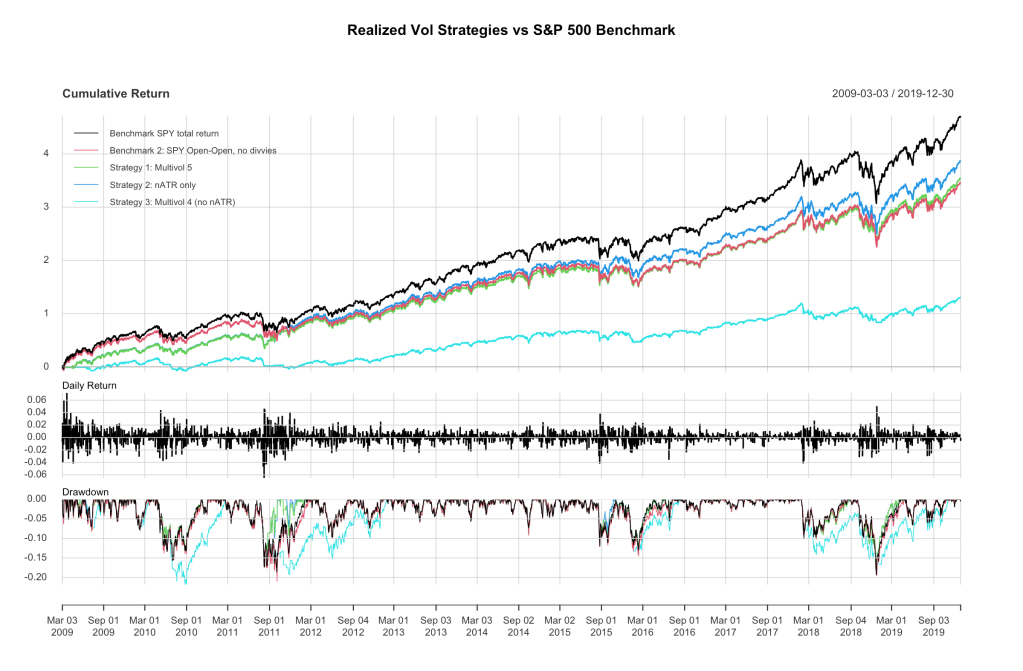
Here’s a typical backtest plot from the updated quant_rv strategy:
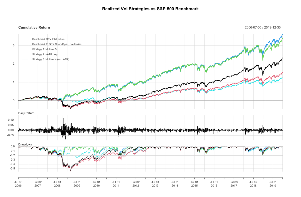
So… wow! Normalized ATR turns out to be a really big player across this time period. Let’s look at the statistics:
| Benchmark SPY Total Return | Benchmark SPY Op-Op | Multivol 5 (with nATR) | nATR alone | Multivol 4 (without nATR) | |
| Annualized Return | 0.0928000 | 0.0714000 | 0.1164000 | 0.1207000 | 0.0636000 |
| Annualized Std Dev | 0.1900000 | 0.1859000 | 0.1599000 | 0.1574000 | 0.1307000 |
| Annualized Sharpe (Rf=0%) | 0.4885000 | 0.3843000 | 0.7278000 | 0.7669000 | 0.4863000 |
| Worst Drawdown | 0.5518944 | 0.5670044 | 0.2168333 | 0.2572825 | 0.2570078 |
Not bad, finally we have a candidate strategy that beats SPY on all our metrics, including Annualized Return. At least, for this select time period it does. Most of the Multivol 5 strategy’s benefit relative to SPY looks like it’s generated during the GFC (late 2008-early 2009) period when SPY really tanked, but quant_rv with nATR was making new highs. Let’s narrow this down and just look at the big bull run from March 2009 to Dec 2019. Another plot and table:
| Benchmark SPY Total Return | Benchmark SPY Op-Op | Multivol 5 (with nATR) | nATR alone | Multivol 4 (without nATR) | |
| Annualized Return | 0.174200 | 0.148000 | 0.1508000 | 0.1582000 | 0.0808000 |
| Annualized Std Dev | 0.156000 | 0.151600 | 0.1418000 | 0.1410000 | 0.1253000 |
| Annualized Sharpe (Rf=0%) | 1.116500 | 0.976300 | 1.0632000 | 1.1220000 | 0.6447000 |
| Worst Drawdown | 0.193489 | 0.209528 | 0.1820016 | 0.1820016 | 0.2181998 |
Yes, it’s clear that quant_rv falls a bit short during a long bull run. The Multivol 5 approach seems geared toward avoiding the big market swoons, but struggles to keep up with a buy-and-hold strategy the rest of the time. Multivol 4 (the previous quant_rv strategy) lags far behind the benchmarks, but Multivol 5 with nATR lags far less. I think clearly adding nATR to quant_rv is helping to reach our goals.
One more plot: 20 random Multivol 5 quant_rv equity curves overlain on one plot, along with the SPY Total Return benchmark.
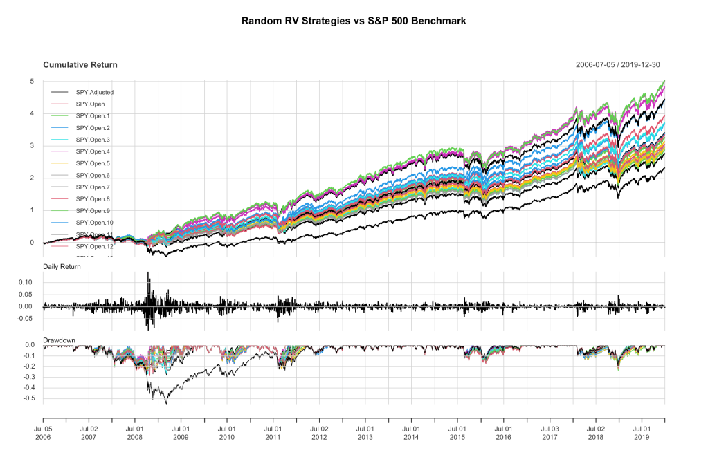
I’ve rerun the code for this a number of times, and this version is pretty good at showing the range of most runs, with the lowest returns in the range of 9-10% CAGR (SPY here is 9.3%) and the highest returns above 14%. Some other stats:
| Stat | Multivol 5 | SPY Total Return |
| Standard deviation | 14.9% to 16.2% | 19% |
| Market exposure | 91-95% | 100% |
| Sharpe ratio | 0.66 to 0.89 | 0.49 |
| Maximum drawdown | -19% to -29% | -55% |
Ok, I’ll wrap this up by saying quant_rv is making progress. I don’t want to jump up and down and yell “Success! We frakkin’ beat SPY and met all our goals!” because something could still blow up, and there’s always a caveat somewhere lurking. However, I can say this seems a reasonable, logical strategy based on SPY volatility that beats the SPY benchmark both in risk-adjusted and unadjusted terms, at least with backtesting over the time period shown. We’ll next explore whether Multivol 5 continues to work before and after this select time period, and what else we might be able to do with it. Beyond that, we’ll continue exploring this area of research in the hope of building a quant_rv that is even better. Let me know your thoughts in the comments! Code will be posted on Github as well.
Codes are at the GitHub!
Leave a comment