Backtesting quant strategies in R requires paying attention to how we lag() our time series. Here be dragons.
Lagging a time series relative to another is important in many areas, but we use it a lot in backtesting financial strategies. I’ve struggled with the logic of lag() several times, and gotten it wrong more than once. And different packages within the R universe apparently use lag() differently! So this is a note for myself as well as for you, gentle reader, to remind me how lag() works and how we can best use it.
So we’ll start with a little fake stock price data so we can see what we’re lagging. Here’s what the price action looks like:
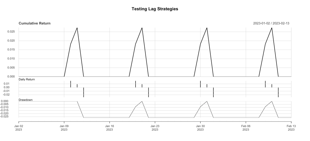
Ok, so that’s not the price action per se, but the daily returns from that fake price sequence. This table (below) shows the first 14 days of data that produced the returns shown in Figure 1. The lagger_0.0.1.R code presented at the bottom produces this model price data.
Date       Open High  Low Close Adj Close Volume

2023-01-01 1.10 1.20 1.00  1.10      1.10      0
2023-01-02 1.10 1.20 1.00  1.10      1.10      0
2023-01-03 1.10 1.20 1.00  1.10      1.10      0
2023-01-04 1.10 1.20 1.00  1.10      1.10      0
2023-01-05 1.10 1.20 1.00  1.10      1.10      0
2023-01-06 1.10 1.20 1.00  1.10      1.10      0
2023-01-07 1.10 1.20 1.00  1.10      1.10      0
2023-01-08 1.10 1.20 1.00  1.10      1.10      0
2023-01-09 1.10 1.20 1.00  1.10      1.10      0
2023-01-10 1.12 1.22 1.02  1.12      1.12      0
2023-01-11 1.13 1.23 1.03  1.13      1.13      0
2023-01-12 1.10 1.20 1.00  1.10      1.10      0
2023-01-13 1.10 1.20 1.00  1.10      1.10      0
2023-01-14 1.10 1.20 1.00  1.10      1.10      0
It’s about 50 bars of pricing, every tenth bar the price goes up sharply, then up slightly more the next day, then back to where it started on the third day. Since that’s such a pretty pattern, we’ll seize the edge it offers and craft a strategy to capture it… when we see the daily ROC go over a threshold of 0.015, we’ll invest for the next day to capture the small secondary rise. And here’s what that looks like:
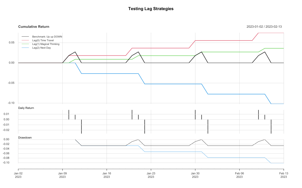
The benchmark is familiar… same as in Figure 1, rescaled. Now because there are no weekends in our fake data, and it starts on Jan 1, that means Jan 10 is our first day where the signal (in black) passes the threshold (0.015) and returns 1 (TRUE). Now here is where the lag() function comes in. I’ll drop the full code below and in Github, but here’s a modified snippet:
# here's the signal, we go long when 1-day ROC at the close is above threshold
signal <- ifelse(roc_close >= roc_thresh, 1, 0)

# and here we calculate the return, adding a 1-day lag to the signal
returns_strategy1 <- roc_trade * stats::lag(signal, 1)

# remove pesky NAs, just because we can
returns_strategy1 <- na.omit(returns_strategy1)
Now we have to talk this through. The signal == 1 on Jan 10 at the close of the market, and that signal was the ROC from Jan 9 to Jan 10, when the market went up about 2%, easily passing our 0.015 threshold. If you squint and read the legend on Figure 2, you’ll see that there are three strategies that differ ONLY in the amount of lag(x) applied to the return stream: 0 lag, 1-day lag and 2-day lag. You can also see in Figure 2 that there are very clear differences in the strategy equity curves. Lag(0) captures only the big Up moves, lag(1) captures only the smaller, trailing up moves, and lag(2) catches only the nosedives. For all four cycles on the plot. Let’s reason this out and see why.
Let’s start with lag(0). This simply means that the return (1-day ROC) from our strategy is the same return as we saw in the daily signal, we’re using the Day 10 signal to capture the Day 10 returns. So even though our signal is coming at the close of the market, somehow we’re going back in time 24 hours (daily bars) and investing at yesterday’s close to get today’s 1-day return! That’s why the first equity curve is labeled “Lag(0) Time Travel”. You can’t do that, not with current technology, so we have to lag our returns.
The next one is called “Lag(1) Magical Thinking”. That’s because you have to use sleight of hand to actually use it. Lag(1) means we use our Day 10 signal to catch the Day 11 returns. That means we have to measure the signal at 10 seconds before the close, and put in our order to buy at the close on Day 10, so we can capture the 1-day return for Day 11. As long as you’re always available at 3:59:50 pm New York time, this can work, but that’s why it’s called “Magical Thinking”. Or if your algo-machine can do it for you. Most days you’re pretty sure by 3:45 if you’re going to be over a simple threshold like this, so it’s mostly achievable, with some semi-acceptable tracking error with respect to the real close. But it’s still magical thinking, because you’ll never be able to use the daily close before it closes, or catch the daily close with your trade.
The final one is called Lag(2) Next Day, because you go into the market at the next close (the close following the one that gave you your signal), so that means we get the signal on Jan 10, and go long at the close on Jan 11, and get the 1-day return measured at the close on Jan 12. Which just sucks.
Now all of that ONLY applies to trading at the close. We can also choose to trade at the open each day, which is easier. Market closes on Jan 10 and the signal is given, so you invest at the morning’s open on Jan 11 and get out again at the open on Jan 12. So what is our lag to reproduce this strategy?
Exactly what you feared. Lag(2) Next Day is what you need, and with this data you capture the downswing, the nosedive, the perfect sequence of losses shown above. Lag(1) for trading on the next open would mean you invest at the open on Jan 10, and sell at the open on Jan 11, but that’s not even magical thinking, that’s just time travel, and it would only net you the smaller, second day gains. Lag(0) is two day back time travel, even harder to accomplish, except with backtesting software.
To my way of thinking, this is time travel back in time, because I try to actually live outside the algorithm and think of this issue as “when do I invest to achieve the same results as this lag() function gives me”. Many quants think of this in the other sense, as a kind of “future-peeking”. I think they must be living inside the algorithm and the calculated return stream, and thinking “Oh, these results are too good, I must be future-peeking somewhere.” If you use the term “future-peeking”, you’re probably living in the algorithm. In any case, pay attention to your lagging and don’t fall for the “Biff Tanner” logical error.
This is demo data, not real, and the Up-up-DOWN nature of this data was selected to provide particularly heinous returns. Unless you’re a time traveler. In the real world, there are some strategies where a signal-at-the-close-lag(2)-invest-at-the-open can work. That’s what I’m striving for with quant_rv. And I think I’m making headway toward it.
Full code for the strategy is here below, and at the Github. Comments welcome.
### lagger v0.0.1 by babbage9010 and friends
### released under MIT License
#
# Simple backtesting demo to understand how lag() works
#

# Load the necessary libraries
library(quantmod)
library(PerformanceAnalytics)

# Generate date sequence from Jan 1, 2023 to Feb 28, 2023
dates <- seq(from = as.Date("2023-01-01"), to = as.Date("2023-02-13"), by = "days")

# Create a matrix with labeled columns
data_matrix <- matrix(
  c(1.1, 1.2, 1.0, 1.1, 1.1, 0),
  nrow = length(dates),
  ncol = 6,
  byrow = TRUE,
  dimnames = list(dates, c("Open", "High", "Low", "Close", "Adjusted Close", "Volume"))
)

# Create the XTS object
my_xts <- xts(data_matrix, order.by = dates)

# Apply the specified pattern to the relevant columns
for (i in seq_along(my_xts[,1])) {
  if (i %% 10 == 0 && i > 3) {
    # Every 10th day: Increase Open, High, Low, Close, Adjusted Close by 0.02
    my_xts[i, c("Open", "High", "Low", "Close", "Adjusted Close")] <- my_xts[i, c("Open", "High", "Low", "Close", "Adjusted Close")] + 0.02
  } else if ((i - 1) %% 10 == 0 && i > 3) {
    # The day after the 10th day: Increase Open, High, Low, Close, Adjusted Close by 0.01
    my_xts[i, c("Open", "High", "Low", "Close", "Adjusted Close")] <- my_xts[i, c("Open", "High", "Low", "Close", "Adjusted Close")] + 0.03
  }
}


#strategy
prices_close <- Ad(my_xts)
prices_open <- Op(my_xts)
roc_close <- ROC(prices_close, n = 1, type = "discrete")
roc_open <- ROC(prices_open, n = 1, type = "discrete")

returns_benchmark <- roc_close
returns_benchmark <- na.omit(returns_benchmark)

comparison1 <- cbind(returns_benchmark)
colnames(comparison1) <- c("Benchmark: Up up DOWN")
charts.PerformanceSummary(comparison1, main = "Testing Lag Strategies")

#strategies testing lag
roc_thresh <- 0.015

roc_trade <- roc_open #substitute roc_close to look at the close!
signal <- ifelse(roc_close >= roc_thresh, 1, 0)

#lag(0)
returns_strategy0 <- roc_trade * stats::lag(signal, 0)
returns_strategy0 <- na.omit(returns_strategy0)

#lag(1)
returns_strategy1 <- roc_trade * stats::lag(signal, 1)
returns_strategy1 <- na.omit(returns_strategy1)

#lag(2)
returns_strategy2 <- roc_trade * stats::lag(signal, 2)
returns_strategy2 <- na.omit(returns_strategy2)

comparison2 <- cbind(returns_benchmark, returns_strategy0, returns_strategy1, returns_strategy2)
colnames(comparison2) <- c("Benchmark: Up up DOWN", "Lag(0) Time Travel", "Lag(1) Magical Thinking", "Lag(2) Next Day")
stats_rv <- rbind(table.AnnualizedReturns(comparison2), maxDrawdown(comparison2))
charts.PerformanceSummary(comparison2, main = "Testing Lag Strategies")
final note: different versions of lag()
When I fire up R Studio and run code containing a lag() function call, it gives me a warning about dplyr::lag() vs stats::lag() and offers some helpful suggestions. Because in my quant_rv code I’m always using XTS objects, I specify stats:lag() because it deals with time series data by default. For my use cases, I haven’t seen any outcome differences between using dplyr::lag() vs stats, but I’ve not tested it extensively. I’ve gleaned from various posts that if you’re tidier than I am and working within dataframes, then you should likely be using dplyr::lag() instead. Caveat emptor, YMMV, good luck, thanks for reading.
addendum: examine your lag()
In a real backtesting strategy, looking for lag issues isn’t always so easy. But one way to do it is to build a comparison XTS object with different lag versions to examine. In this code, we build “comparison2” consisting of the benchmark returns and the three lagged strategy returns. By simply viewing the comparison2 object in R Studio, you can quickly see the differences among the three lags and how lag() works here:
Date      Up up DOWN   Lag(0)   Lag(1)    Lag(2)
2023-01-08   0.00000  0.00000  0.00000   0.00000
2023-01-09   0.00000  0.00000  0.00000   0.00000
2023-01-10   0.01818  0.01818  0.00000   0.00000
2023-01-11   0.00893  0.00000  0.00893   0.00000
2023-01-12  -0.02655  0.00000  0.00000  -0.02655
2023-01-13   0.00000  0.00000  0.00000   0.00000
2023-01-14   0.00000  0.00000  0.00000   0.00000
Again, the signal comes in at the close on Jan 10. Lag(0) nets the same return as triggered the signal (Time Travel required if trading at the close or the next open). Lag(1) nets the lesser move upward, but requires a Magical Thinking trade at the same close that generates the signal; achieving lag(1) results with trading the open again requires Time Travel back to the opening bell on Jan 10. Lag(2) nets the price drop return, and is appropriate for using the signal from Jan 10 to invest at the next day open or the next day close.
Hope that makes lagging clearer!

Leave a comment