In recent posts we added nATR as a vol measure, went short instead of flat, and significantly improved quant_rv’s performance over our in-sample test period 2006-2019. Now we look at the more recent record including the Covid Swoon and Inflation Coaster, and the years prior from the Roaring 90s through the Dot Com Crash. Short take: this was not a strategy anyone would have chosen before the Great Financial Crisis of 2008-2009. A good question is… why?
We’ve been working on quant_rv for the period 2006/07/01 to 2019/12/31. We have a strategy that beats SPY soundly on all measures. But we’ve not explored the time period since then or before. Let’s fix that now.
First up, let’s look at the more recent update… is quant_rv still working today? Here’s a plot for ya:
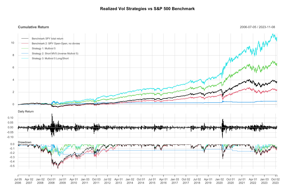
Yup, it’s still working. In early 2020 we had the Covid Swoon which was used to advantage by quant_rv. Then we ran up and up along with Mr. Market through the end of 2021 until the Inflation Rollercoaster started downhill. Performance has been choppy, but clearly better than SPY which still hasn’t broken out of the doldrums. The Long/Short version returns 15.4% annually on this run, compared with 9.4% for SPY.
For completion, we can run our 20-curve Randomized Monte Carlo plot to see the range of equity curves quant_rv might have generated in live action, and…
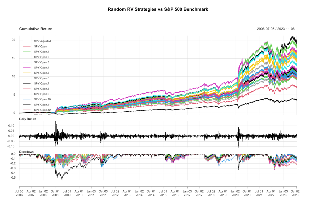
…we can see that the Figure 1 run was in the middle of the pack. Some of the curves look no better than SPY for the Inflation Rollercoaster, but none seem worse. We see annual returns ranging from 13-19% with no big failures anywhere.
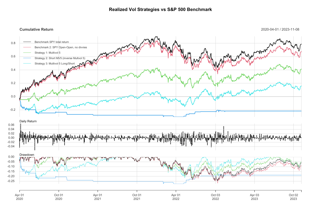
Or do we? Let’s start this run near the low point of the Covid Swoon, say April 1, 2020. Now we’re seeing some failure!
Now I’ve made this look about as bad as it can be. If I started two months earlier, you’d see a good kick upward for the short leg as the Covid Swoon hit the markets, and then this failure wouldn’t look quite so bad. Oh heck, I’ll just show you what I mean, here’s the plot from February onward.
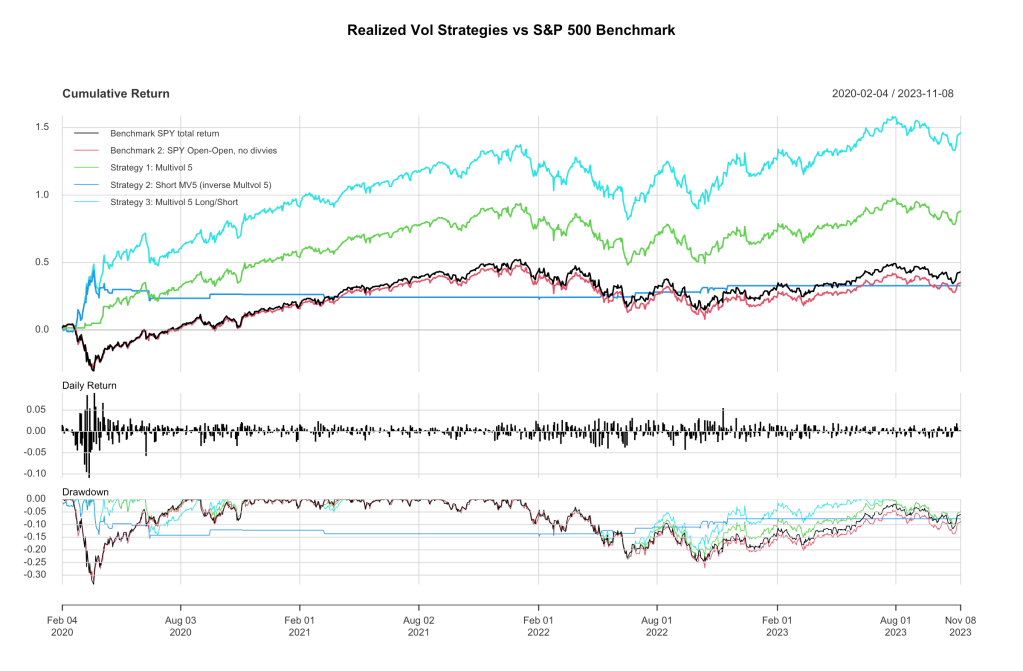
There, see? As Covid hysteria took the markets down, vol shot through the roof and quant_rv went short SPY (or long SH) and did great. The short leg was super helpful here, but then high vol overshot the market low and our short leg lost a good bit of its gain over the next few months as the market responded to all the stimulus.
So overall, not a failure for these last few years. quant_rv overall seems to be modestly underpowered during bull times and hyperdriven during market plunges. It doesn’t seem to be doing anything wonderful through these Inflation Rollercoaster times we have now, but it’s not failing miserably either. Overall, it’s a fairly successful long-term strategy for the past 17 years, avoiding the big losses and in fact turning them into big wins to beat the market overall.
Trouble behind
The trouble is, nobody would have started this strategy in 2006. There was nothing in the past that would tell you to do so. There was no low volatility anomaly in SPY (as defined in recent posts) prior to 2006. Let’s take a look.
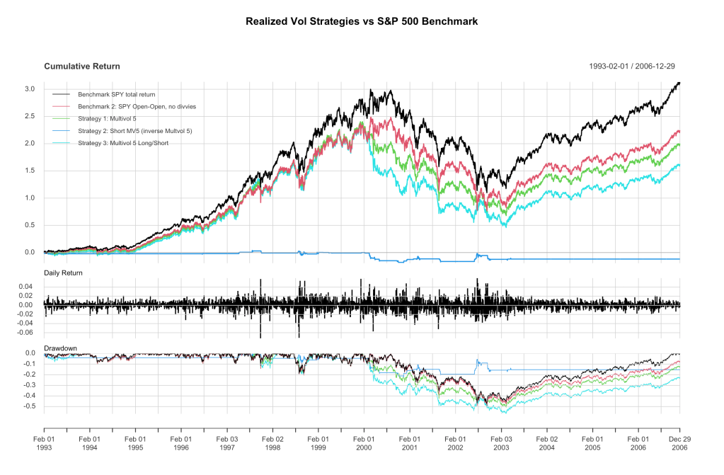
Fairly unspectacular results, basically what you’d expect for a random 90% market exposure strategy, until around Feb 2000 when market vol went sky high just before the Dot Com Bust and quant_rv started it’s drawdown well before the market did, and just kept going. Pretty ugly actually.
And that’s because… there was no low vol anomaly. We can run the other volatility/lookback comparison plots from our other posts for all five of the vol measures over this time period and the short of it is there was NO low volatility anomaly in SPY over that time. You can substitute ^GSPC into the code instead of SPY and take it back through the eighties and there’s still no anomaly.
Actually, there is one bright spot: this exercise is left to the reader, but quant_rv manages to do fairly well through the Black Friday fiasco in October 1987, but that’s the only nice thing that can be said for this four decade retrospective.
why, Babbage? why?
So why is there a low vol anomaly now, when there wasn’t one before? I think there are at least two reasons. First is the rise in ETF trading volume and systematic usage by retirement funds, and second is the rise in volatility-targeting fund strategies. Both of these contribute to “virtuous cycles” of market gains begetting lower volatility begetting further leveraging up and market gains begetting yet lower volatility. Until they don’t and vol shoots up and markets correct. And then it starts again.
For some of you readers, that’s a gross oversimplification or even misstatement. For others it may be unintelligible or worse. I’m only aping what I’ve read, and this explanation may even be insulting to the apes. But I’ll try. Let’s talk about vol-targeting funds and how their rise (~perhaps half a $trillion or more today) could contribute to a low volatility SPY anomaly. Vol-targeting means the fund has a target volatility for its portfolio. So if market volatility goes down, the volatility for the portfolio goes down too… the fund responds by increasing the leverage on its assets… ie, buy more assets on margin, to keep volatility at the higher target level. So, you see the feedback more clearly now, right? (Step 1) Market moves up in an orderly fashion and (Step 2) market volatility drops, leading to (Step 3) more buying from vol-targeting funds, which provides (Step 4) more demand for assets, which causes (Step 1) market to move up again.
Feedback 101: This is a positive feedback loop, not so-named because it’s a good (positive) thing, but because a directional move triggers feedbacks that cause more movement in the same direction… movement begets more movement leading the system away from some theoretical starting point or equilibrium. A negative feedback loop causes the opposite: directional movement triggers feedback that causes a negative directional movement, back toward the starting measure or some equilibrium point. The thermostat in a room measures temperatures and triggers a negative feedback response if the room gets too hot or too cold.
There’s other possible contributors to a low vol anomaly in SPY. Index ETFs are the elephants in the market nowadays, with about $2 trillion invested in just the top 10 market index funds. Every month like clockwork, money spills into those funds from employees and employers toward retirement dreams, and the funds put that money into the stocks of those companies in the indexes; an orderly push on the demand side helping to move markets upward and dampen market volatility.
I’m going to punt rather than try to delve into what impact a growing options market might have on market volatility. For those of you unfamiliar with American football metaphors, punting means I’m giving YOU the ball to run with it, and offer some suggestions on how options might play a role here. Or make other suggestions as to why there might be a low volatility edge in SPY now when there wasn’t one 20+ years ago. I’m an amateur here, help me out 🙂
PS. No new R code here, just change the start_date or end_date on the previous (v1.3.3) quant_rv code to duplicate these graphs, or try new date ranges. Or substitute “^GSPC” for “SPY” to see how things look with the S&P 500 index back into the early 80s. I will note that if you do this, remember that the code also tries to use the “SH” ETF instead of actually shorting SPY. But SH doesn’t exist before 2006, so instead to simulate what it might have been like to be able to short ^GSPC back in the 1980s, just put ^GSPC into the symbol_trade2 slot, and then set roc_trade2 to -1 * ROC(prices_trade2, n = 1, type = “discrete”), et voilà.
Thanks for reading.
~babbage

Leave a comment